
What is OpenBB
OpenBB is an open-source platform that integrates more than 100 different data sources, across all asset classes, from stocks, options, crypto assets, forex, macroeconomic data, and much more. It offers access options from a Bloomberg-style app, an old Bloomberg-style CLI console, and leaves the door open to Python programmers through its openbb package.
Historically, accessing financial data was a considerable challenge—it was expensive, inaccessible, and required too much time. With OpenBB, they simplify this entire process by centralizing all data sources in a single point. Using a single library to obtain all our data in real time.
Installing the necessary libraries
Using the Dockerized stack we created
 quantarmyz
we load the environment we use from a terminal, and run the following command, which will install the Python gateway that interconnects us with OpenBB, allowing us to work with all the power of OpenBB from Python in an extremely simple way.

!pip install openbb[all]
First Use of OpenBB
Once the library is downloaded, loading the library in Python for the first time will download and install some additional packages in the background.
from openbb import obb
obb.user.preferences.output_type = 'dataframe'
Once finished, it is recommended to restart the kernel, and the library will be fully functional.
Getting Stock Data
Comparing Fundamental Data
obb.equity.fundamental.metrics("AAPL,MSFT").T
| 0 | 1 | |
|---|---|---|
| symbol | AAPL | MSFT |
| market_cap | 3414690000000.0 | 3109760000000.0 |
| pe_ratio | 34.2 | 35.45 |
| foward_pe | 30.26 | 27.23 |
| eps | 6.57 | 11.8 |
| price_to_sales | 8.86 | 12.69 |
| price_to_book | 51.25 | 11.58 |
| book_value_per_share | 4.38 | 36.11 |
| price_to_cash | 55.25 | 41.17 |
| cash_per_share | 4.06 | 10.16 |
| price_to_free_cash_flow | 32.73 | 41.98 |
| debt_to_equity | 1.52 | 0.36 |
| long_term_debt_to_equity | 1.29 | 0.31 |
| quick_ratio | 0.91 | 1.27 |
| current_ratio | 0.95 | 1.27 |
| gross_margin | 0.4596 | 0.6976 |
| profit_margin | 0.2644 | 0.3596 |
| operating_margin | 0.3127 | 0.4464 |
| return_on_assets | 0.3059 | 0.1907 |
| return_on_investment | 0.6668 | 0.2508 |
| return_on_equity | 1.6058 | 0.3713 |
| payout_ratio | 0.1532 | 0.2542 |
Price Data
data = obb.equity.price.historical("SPY")
If we want to change the timeframe, we do it through the interval parameter:
1m= One Minute1h= One Hour1d= One Day1W= One Week1M= One Month
In this case, we leave it by default, on a daily timeframe.
| open | high | low | close | volume | |
|---|---|---|---|---|---|
| date | |||||
| 2004-01-02 | 111.74 | 112.19 | 110.73 | 111.23 | 38072300 |
| 2004-01-05 | 111.69 | 112.52 | 111.59 | 112.44 | 27959800 |
| 2004-01-06 | 112.16 | 112.73 | 112.00 | 112.55 | 20472800 |
| 2004-01-07 | 112.39 | 113.06 | 111.89 | 112.93 | 30170400 |
| 2004-01-08 | 113.25 | 113.41 | 112.77 | 113.38 | 36438400 |
| ... | ... | ... | ... | ... | ... |
| 2024-09-25 | 571.19 | 571.89 | 568.91 | 570.04 | 37682308 |
| 2024-09-26 | 574.49 | 574.71 | 569.90 | 572.30 | 44788926 |
| 2024-09-27 | 573.42 | 574.22 | 570.42 | 571.47 | 41082707 |
| 2024-09-30 | 570.50 | 574.38 | 568.08 | 573.76 | 59333099 |
| 2024-10-01 | 573.41 | 574.06 | 566.00 | 568.62 | 70827736 |
5227 rows × 5 columns
Comparing Sectors Fundamentally
obb.equity.compare.groups(group="industry",metric="valuation").T
| 0 | 1 | 2 | 3 | 4 | 5 | 6 | 7 | 8 | 9 | ... | 135 | 136 | 137 | 138 | 139 | 140 | 141 | 142 | 143 | 144 | |
|---|---|---|---|---|---|---|---|---|---|---|---|---|---|---|---|---|---|---|---|---|---|
| name | Pharmaceutical Retailers | Insurance - Reinsurance | REIT - Mortgage | Coking Coal | Airlines | Marine Shipping | Financial Conglomerates | Insurance - Life | Paper & Paper Products | Thermal Coal | ... | Biotechnology | REIT - Industrial | REIT - Specialty | Uranium | REIT - Residential | REIT - Office | REIT - Healthcare Facilities | Shell Companies | Real Estate - Diversified | Infrastructure Operations |
| market_cap | 7980000000 | 50930000000 | 58520000000 | 10270000000 | 126700000000 | 40150000000 | 35370000000 | 300640000000 | 17030000000 | 11610000000 | ... | 1302310000000 | 301390000000 | 425450000000 | 33400000000 | 201730000000 | 76590000000 | 163750000000 | 27320000000 | 7570000000 | 34940000000 |
| performance_1D | 0.0232 | 0.0024 | -0.001 | 0.005 | -0.0179 | 0.0052 | -0.0036 | 0.0117 | 0.0077 | 0.0107 | ... | -0.0119 | -0.0122 | -0.0031 | 0.0214 | -0.0066 | -0.0011 | -0.0055 | -0.0018 | 0.0002 | -0.0111 |
| forward_pe | 5.1 | 7.2 | 7.45 | 7.71 | 8.08 | 8.43 | 9.04 | 9.07 | 9.41 | 9.49 | ... | 35.87 | 39.97 | 41.55 | 47.82 | 49.76 | 56.3 | 66.47 | 138.44 | 147.61 | 151.85 |
| eps_growth_past_5_years | -0.0482 | 0.5531 | -0.2214 | 0.0583 | -0.0431 | 0.2148 | 0.0292 | -0.0107 | 0.7162 | 0.1513 | ... | 0.0123 | 0.0735 | 0.1308 | 0.1901 | 0.1472 | -0.2137 | -0.1288 | NaN | 0.1838 | NaN |
| eps_growth_next_5_years | 0.0569 | 0.0746 | 0.0313 | 0.0626 | 0.1492 | 0.0992 | 0.1386 | 0.0891 | 0.0839 | -0.0487 | ... | 0.1187 | 0.0181 | 0.1124 | NaN | 0.0175 | 0.0068 | 0.3635 | NaN | 0.1975 | 0.1425 |
| sales_growth_past_5_years | 0.0371 | 0.2218 | 0.3533 | 0.1565 | 0.2438 | 0.2487 | -0.0061 | 0.0554 | 0.1615 | 0.1014 | ... | 2.8221 | 0.192 | 1.1581 | 2.5959 | 0.0841 | 0.0651 | 0.1157 | 0.6025 | 0.2097 | 0.0814 |
| volume | 3530000 | 115690 | 6380000 | 155130 | 11860000 | 3030000 | 286490 | 1810000 | 211010 | 326830 | ... | 89480000 | 1480000 | 2089999 | 9190000 | 1720000 | 1920000 | 3610000 | 1020000 | 27680 | 95120 |
| price_to_sales | 0.05 | 0.95 | 1.84 | 0.97 | 0.47 | 1.33 | 1.22 | 1.14 | 0.99 | 1.16 | ... | 10.21 | 12.22 | 7.39 | 13.47 | 8.28 | 3.93 | 7.08 | 26.2 | 4.81 | 3.34 |
| price_to_book | 0.57 | 1.31 | 0.88 | 1.67 | 2.16 | 1.14 | 1.19 | 1.66 | 1.84 | 1.42 | ... | 5.37 | 2.73 | 6.48 | 4.31 | 2.66 | 1.11 | 2.11 | 2.39 | 1.93 | 7.74 |
| price_to_cash | 9.77 | NaN | 4.17 | 7.11 | 2.3 | 6.33 | 3.38 | 3292.14 | 3.83 | 9.08 | ... | 6.7 | 127.49 | 42.58 | 22.22 | 56.66 | 8.74 | 30.35 | 40.93 | 7.39 | 8.61 |
| price_to_free_cash_flow | 419.39 | 2.85 | 6.73 | 9.71 | 28.04 | 9.46 | 3.74 | 4.88 | 25.63 | 6.79 | ... | 48.67 | 25.91 | 44.93 | 98.93 | 23.16 | 13.92 | 28.53 | 109.4 | 72.23 | 33.73 |
| pe | NaN | 7.01 | 24.3 | 8.37 | 12.11 | 6.31 | 11.01 | 13.83 | 49.52 | 7.37 | ... | 55.96 | 41.22 | 46.15 | 88.93 | 44.87 | 88.88 | 112.84 | 58.46 | 95.48 | 38.81 |
| peg | NaN | 0.94 | 7.77 | 1.34 | 0.81 | 0.64 | 0.79 | 1.55 | 5.9 | NaN | ... | 4.72 | 22.75 | 4.11 | NaN | 25.58 | 130.73 | 3.1 | NaN | 4.83 | 2.72 |
14 rows × 145 columns
Derivatives: Data from a Futures Curve
data = obb.derivatives.futures.curve(symbol="VX")
| expiration | price | |
|---|---|---|
| 0 | 2024-10 | 20.50 |
| 1 | 2024-11 | 19.35 |
| 2 | 2024-12 | 18.90 |
| 3 | 2025-01 | 19.30 |
| 4 | 2025-02 | 19.50 |
| 5 | 2025-03 | 19.60 |
| 6 | 2025-04 | 19.65 |
| 7 | 2025-05 | 19.75 |
| 8 | 2025-06 | 19.85 |
Plotting the curve
import pandas as pd
data.index = pd.to_datetime(data.expiration)
data.plot()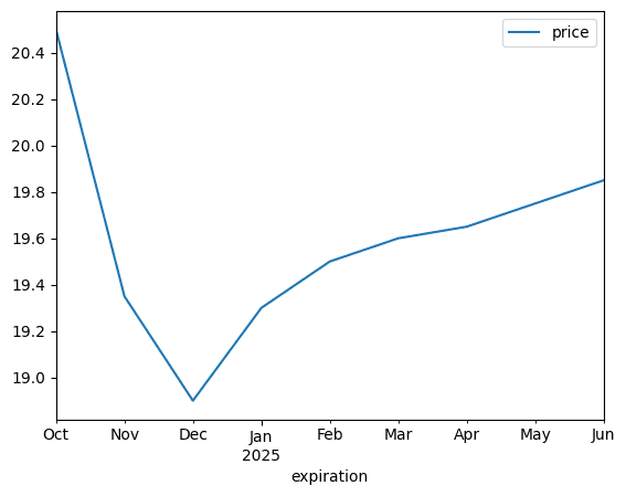
Download and plot different contracts
expirations = [
    "2024-12",
    "2025-12",
    "2026-12",
    "2027-12",
    "2028-12",
    "2029-12",
    "2030-12",
]
contracts = []
for expiration in expirations:
df = (
obb
.derivatives
.futures
.historical(
symbol="CL",
expiration=expiration,
start_date="2020-01-01",
end_date="2022-12-31"
)
).rename(columns={
"close": expiration
})
contracts.append(df[expiration])historical = (
pd
.DataFrame(contracts)
.transpose()
.dropna()
)
historical.plot()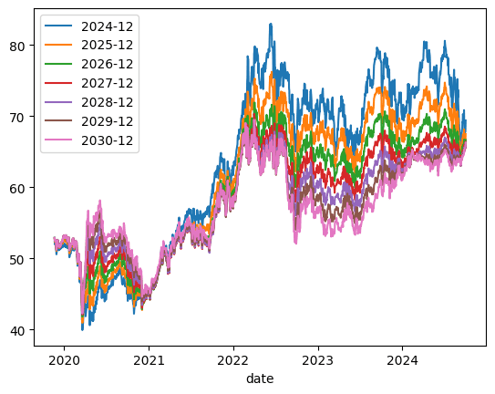
Getting an Options Chain
Regarding the options chain, we will cover it separately in a future article, exploring all the possibilities that OpenBB provides. For now, to snapshot the current chain of a specific ticker, it would be done as follows:
chains = obb.derivatives.options.chains(symbol="SPY")| underlying_symbol | underlying_price | contract_symbol | expiration | dte | strike | option_type | open_interest | volume | theoretical_price | ... | low | prev_close | change | change_percent | implied_volatility | delta | gamma | theta | vega | rho | |
|---|---|---|---|---|---|---|---|---|---|---|---|---|---|---|---|---|---|---|---|---|---|
| 0 | SPY | 568.1201 | SPY241002C00300000 | 2024-10-02 | 0 | 300.0 | call | 5 | 12 | 268.1850 | ... | 268.16 | 269.485001 | -0.725 | -0.00269 | 0.0000 | 1.0000 | 0.0000 | -0.0024 | 0.0000 | 0.0000 |
| 1 | SPY | 568.1201 | SPY241002P00300000 | 2024-10-02 | 0 | 300.0 | put | 10 | 0 | 0.0001 | ... | 0.00 | 0.005000 | 0.000 | 0.00000 | 7.0620 | 0.0000 | 0.0000 | -0.0001 | 0.0000 | 0.0000 |
| 2 | SPY | 568.1201 | SPY241002C00310000 | 2024-10-02 | 0 | 310.0 | call | 0 | 0 | 258.1850 | ... | 0.00 | 259.535004 | 0.000 | 0.00000 | 0.0000 | 1.0000 | 0.0000 | -0.0024 | 0.0000 | 0.0000 |
| 3 | SPY | 568.1201 | SPY241002P00310000 | 2024-10-02 | 0 | 310.0 | put | 0 | 0 | 0.0002 | ... | 0.00 | 0.005000 | 0.000 | 0.00000 | 6.7156 | 0.0000 | 0.0000 | -0.0002 | 0.0000 | 0.0000 |
| 4 | SPY | 568.1201 | SPY241002C00320000 | 2024-10-02 | 0 | 320.0 | call | 0 | 0 | 248.1850 | ... | 0.00 | 249.514999 | 0.000 | 0.00000 | 0.0000 | 1.0000 | 0.0000 | -0.0024 | 0.0000 | 0.0000 |
| ... | ... | ... | ... | ... | ... | ... | ... | ... | ... | ... | ... | ... | ... | ... | ... | ... | ... | ... | ... | ... | ... |
| 9863 | SPY | 568.1201 | SPY270115P00890000 | 2027-01-15 | 835 | 890.0 | put | 0 | 0 | 321.8150 | ... | 0.00 | 320.589996 | 0.000 | 0.00000 | 0.2833 | -1.0000 | 0.0000 | -0.0640 | 0.0000 | 0.0000 |
| 9864 | SPY | 568.1201 | SPY270115C00895000 | 2027-01-15 | 835 | 895.0 | call | 0 | 0 | 0.8942 | ... | 0.00 | 0.875000 | 0.000 | 0.00000 | 0.1243 | 0.0253 | 0.0006 | -0.0034 | 0.5654 | 0.2984 |
| 9865 | SPY | 568.1201 | SPY270115P00895000 | 2027-01-15 | 835 | 895.0 | put | 0 | 0 | 326.8150 | ... | 0.00 | 325.589996 | 0.000 | 0.00000 | 0.2861 | -1.0000 | 0.0000 | -0.0640 | 0.0000 | 0.0000 |
| 9866 | SPY | 568.1201 | SPY270115C00900000 | 2027-01-15 | 835 | 900.0 | call | 225 | 0 | 0.8464 | ... | 0.00 | 0.925000 | 0.000 | 0.00000 | 0.1265 | 0.0240 | 0.0005 | -0.0033 | 0.5430 | 0.2836 |
| 9867 | SPY | 568.1201 | SPY270115P00900000 | 2027-01-15 | 835 | 900.0 | put | 0 | 0 | 331.8150 | ... | 0.00 | 330.589996 | 0.000 | 0.00000 | 0.2888 | -1.0000 | 0.0000 | -0.0640 | 0.0000 | 0.0000 |
9868 rows × 29 columns
Downloading a specific option
If within the chain we want to download a specific contract, we must treat it as if we were downloading a stock ticker, but the symbol is the option identifier. As follows:
data = obb.equity.price.historical(
    symbol="SPY241220C00550000",
provider="yfinance")| open | high | low | close | volume | split_ratio | dividend | |
|---|---|---|---|---|---|---|---|
| date | |||||||
| 2023-10-02 | 2.340000 | 2.340000 | 2.140000 | 2.140000 | 1004 | 0.0 | 0.0 |
| 2023-10-03 | 2.240000 | 2.240000 | 2.010000 | 2.030000 | 47 | 0.0 | 0.0 |
| 2023-10-04 | 2.050000 | 2.200000 | 2.050000 | 2.200000 | 4 | 0.0 | 0.0 |
| 2023-10-06 | 2.030000 | 2.600000 | 2.030000 | 2.600000 | 26 | 0.0 | 0.0 |
| 2023-10-09 | 2.500000 | 2.780000 | 2.500000 | 2.780000 | 19 | 0.0 | 0.0 |
| ... | ... | ... | ... | ... | ... | ... | ... |
| 2024-09-26 | 37.959999 | 37.980000 | 35.630001 | 36.500000 | 30 | 0.0 | 0.0 |
| 2024-09-27 | 36.790001 | 36.790001 | 35.880001 | 35.939999 | 32 | 0.0 | 0.0 |
| 2024-09-30 | 35.500000 | 37.480000 | 33.799999 | 37.480000 | 21 | 0.0 | 0.0 |
| 2024-10-01 | 35.619999 | 35.619999 | 33.090000 | 34.660000 | 62 | 0.0 | 0.0 |
| 2024-10-02 | 32.570000 | 32.570000 | 32.570000 | 32.570000 | 2 | 0.0 | 0.0 |
246 rows × 7 columns
Forex
obb.currency.price.historical("usdjpy", provider="yfinance").to_df()| open | high | low | close | volume | |
|---|---|---|---|---|---|
| date | |||||
| 2023-08-22 | 146.238007 | 146.389999 | 145.501999 | 146.238007 | 0.0 |
| 2023-08-23 | 145.763000 | 145.813004 | 144.580002 | 145.763000 | 0.0 |
| 2023-08-24 | 144.673004 | 145.947006 | 144.621002 | 144.673004 | 0.0 |
| 2023-08-25 | 146.067001 | 146.604996 | 145.733994 | 146.067001 | 0.0 |
| 2023-08-28 | 146.531006 | 146.716003 | 146.278000 | 146.531006 | 0.0 |
| ... | ... | ... | ... | ... | ... |
| 2024-08-16 | 149.222000 | 149.229996 | 147.639008 | 149.222000 | 0.0 |
| 2024-08-19 | 147.955994 | 147.959000 | 145.220993 | 147.955994 | 0.0 |
| 2024-08-20 | 146.699005 | 147.319000 | 145.533997 | 146.699005 | 0.0 |
| 2024-08-21 | 145.347000 | 146.339005 | 144.981003 | 145.347000 | 0.0 |
| 2024-08-22 | 145.117996 | 146.524994 | 144.839996 | 146.287003 | 0.0 |
Data Validation
As an extra, we are going to compare data from different providers to get an approximation of the quality of the data we are managing. Data is the input of the process, and low-quality raw material will generate low-quality models. For this test, we will verify the volume on the QQQ ticker (Nasdaq Composite ETF).
To validate that the data from the different providers is correct, we should obtain the same volume for all providers.
First, let's collect the necessary data.
yahoo = obb.equity.price.historical("QQQ", provider="yfinance").to_df()
alphavantage = obb.equity.price.historical("QQQ", provider="alpha_vantage").to_df()
intrinio = obb.equity.price.historical("QQQ", provider="intrinio").to_df()
fmp = obb.equity.price.historical("QQQ", provider="fmp").to_df()
polygon = obb.equity.price.historical("QQQ", provider="polygon").to_df()
Using the following code, we download the QQQ ticker from different providers in Pandas DataFrame format.
Now we process the data, creating a new dataframe with the last 10 cases of the volume from the different providers and removing NA values.
compare = pd.DataFrame()
compare["AV Volume"] = alphavantage["volume"].tail(10)
compare["FMP Volume"] = fmp["volume"].tail(10)
compare["Intrinio Volume"] = intrinio["volume"].tail(10)
compare["Yahoo Volume"] = yahoo["volume"].tail(10)
compare["Polygon Volume"] = polygon["volume"].tail(10)

compare.dropna(how="any")| AV Volume | FMP Volume | Intrinio Volume | Yahoo Volume | Polygon Volume | |
|---|---|---|---|---|---|
| date | |||||
| 2024-08-09 | 45619558 | 45619558.0 | 45619558.0 | 45619600.0 | 45425963.0 |
| 2024-08-12 | 42542069 | 42542069.0 | 42542069.0 | 42542100.0 | 42533175.0 |
| 2024-08-13 | 52333073 | 52333073.0 | 52333073.0 | 52333100.0 | 50110167.0 |
| 2024-08-14 | 42446929 | 42446929.0 | 42446929.0 | 42446900.0 | 42362522.0 |
| 2024-08-15 | 60846812 | 60846812.0 | 60846812.0 | 60846800.0 | 60762738.0 |
| 2024-08-16 | 44430728 | 44430728.0 | 44430728.0 | 44430700.0 | 44368969.0 |
| 2024-08-19 | 39121793 | 39121793.0 | 39121793.0 | 39121800.0 | 38648958.0 |
| 2024-08-20 | 33732264 | 33732264.0 | 33732264.0 | 33732300.0 | 33693989.0 |
| 2024-08-21 | 41514600 | 38682509.0 | 41514600.0 | 41467000.0 | 41532360.0 |
As a conclusion, we can see that they do not always match, so everyone must run their own procedures to determine which price is real and which is not.
Conclusions
These short articles aim to get straight to the point This guide is part of the algorithmic trading course, and a Spanish version is also available. in a concentrated way. Through this article, you can access and download time series of different asset classes, to later manage them in our datalake, or in whatever independent way you need.