In the latest installments, we explained seasonality, preprocessed the data, and also started programming a seasonal backtest in python in a simple way. Leaving everything ready for this new installment.
In this new installment, once we have the trades from the trading operations returned by the backtester in a dataframe, we will analyze them. This way we can see at a glance the most relevant statistics of the strategy, also, thinking about the next installment where we will program a broad-spectrum intraday seasonality search module, whose objective is to return a dataframe with the selected parameters and the most relevant statistics.
Other Articles in the Series
 Jesús Cuesta
 Jesús Cuesta
How we will structure it
In the following image, we see how our class will end up. We have already programmed the functions that are inside the red rectangle, which are the main functionalities for searching intraday seasonal patterns.

The objective now will be
- Program the most relevant statistics such as:
- SQN
- VaR & CVaR
- Alpha and Beta
- MDD
- Sharpe Ratio
- Create a summary where it shows us the most relevant information, and which we will later use for the resulting dataframe of the broad-spectrum intraday seasonality search.
Once the objectives are defined, and having explained what we have already done, let's get to it!
SQN - System Quality Number in Python
We are going to program a new function within our class that calculates the SQN on the curve of our strategy.
The System Quality Number (SQN), developed by Dr. Van Tharp, is a statistical metric designed to evaluate the quality and risk-adjusted performance of a trading system.
SQN Formula

Where:
- Mathematical Expectation (E): It is the average expected return per trade in terms of multiples of R (reward/risk ratio).
- Number of Trades (N): Total number of trades made.
- Standard Deviation (DT): Measures the dispersion or variability of R multiples.
Interpretation of the SQN Ratio
Interpretation of SQN
The SQN value indicates the quality of the system:
- < 1.5: Difficult to trade.
- 1.51 - 2.0: Average system.
- 2.01 - 3.0: Good system.
- 3.01 - 5.0: Excellent system.
- 5.01 - 7.0: Outstanding system.
- > 7.0: "Holy Grail" (extremely rare)
Important Considerations
- Sample size: For the SQN to be statistically significant, a minimum of 30 trades is recommended
- Impact of standard deviation: Systems with high variability in results (such as trend-following strategies) tend to have a lower SQN due to their higher standard deviation, even if they are profitable in the long term
- Limitations: SQN can penalize strategies with occasional large gains or positive volatility, making it more favorable for systems with consistent distributions and lower deviations
We are going to create a new function within our class with the following code:
    def calculate_sqn(self,trades=None):
        import numpy as np

        if len(trades) == 0:
            return 0

        avg_trade = trades['Points'].mean()
        std_dev = trades['Points'].std()
        num_trades = len(trades)

        if std_dev == 0:
            return 0

        sqn = (avg_trade / std_dev) * np.sqrt(num_trades)

        return sqn
In the code what we have done is
- Verify that there are Trades
- Subsequently calculate the components of the formula
- And calculate the SQN ratio based on the components
VaR and CVaR
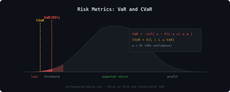
VaR and CVaR are two risk estimators,
$$\text{VaR}_\alpha = -\inf\{x : P(L \leq x) \geq \alpha\}$$
$$\text{CVaR}_\alpha = \mathbb{E}[L \mid L \leq \text{VaR}_\alpha]$$
VaR (Value At Risk)
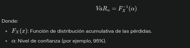
VaR (Value at Risk) measures the maximum loss a portfolio could experience in a specific period, under normal market conditions, with a determined confidence level. In simple terms, VaR answers the question: how much can I lose at most in a given time horizon with a specific probability?
It could be interpreted as if the daily 95% VaR of a portfolio is $1,000,000, it means there is a 5% probability that losses exceed that amount in a day
Formula
Mathematically, VaR is defined as the α percentile of the loss distribution:
Methods for Calculating Value at Risk (VaR)
There are three main methods for calculating VaR:
- Historical simulation: Uses past data to estimate possible future losses
- Variance-covariance method: Assumes that returns have a normal distribution
- Monte Carlo simulation: Generates random scenarios based on statistical models.
Limitations
VaR does not consider the magnitude of losses beyond the defined threshold and can underestimate risk in extreme events (fat tails). Consequently, we must assume that the largest drawdown, or performance loss, is yet to come.
CVaR (Conditional Value At Risk)
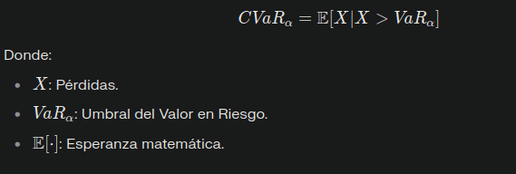
CVaR (Conditional Value at Risk), also known as expected shortfall (Expected Shortfall), complements VaR by measuring the average loss in the worst scenarios that exceed the VaR threshold. Therefore, it provides a more complete view of extreme risk.
For example, if the CVaR at 95% is $1,200,000, it means that within the 5% worst scenarios, the average losses will be $1,200,000
Formula
CVaR is calculated as the average of losses that exceed VaR:
Advantages
CVaR has better mathematical properties than VaR:
- It is a coherent risk measure (satisfies monotonicity, subadditivity, and other properties)
- Better captures extreme risks and allows optimizing portfolios considering adverse scenarios
Programming
We are going to implement Value at Risk and Conditional Value at Risk in the same function as follows:
    def calculate_var_cvar(self, confidence_level=0.95):

        if not self.trades:
            return 0, 0

        if isinstance(self.trades, list):
            trades_df = pd.DataFrame(self.trades)
        else:
            trades_df = self.trades

        r = trades_df['Points'].values

        var = np.percentile(r, (1-confidence_level)*100)
        cvar = r[r <= var].mean() if len(r[r <= var]) > 0 else var

        return var, cvar
First, we verify that trades exist, then we verify that we have them in a dataframe, and if not, we create it ourselves.
We assign to the variable r the values of the variation of our strategy
And we calculate the VaR and CVaR, depositing their results in the variables with the same name and returning them.
The default confidence level is 95, but it is also common to see people who calculate it at the 99% level
Calculating the Greeks (Alpha and Beta)
Alpha
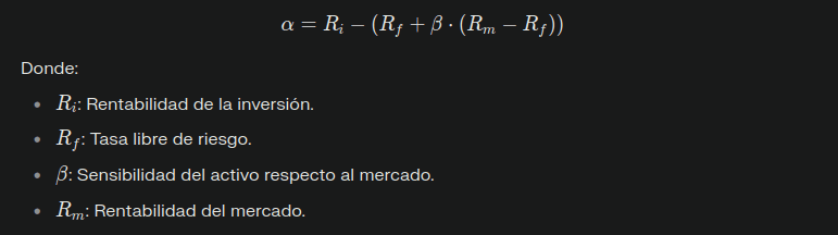
Alpha is a metric that measures the additional performance or "excess return" that an investment generates compared to a reference index (benchmark). In other words, it reflects how much added value (or lost) a portfolio manager or investment strategy contributes beyond the general market behavior.
- A positive Alpha indicates that the investment outperformed the market.
- A negative Alpha implies that the investment underperformed the market.
Formula
Interpretation
- α>0: The investment generated returns above the benchmark adjusted for risk.
- α=0: The investment matched the benchmark's performance.
- α<0: The investment underperformed the benchmark.
Beta
Beta is a measure that quantifies the sensitivity or volatility of an asset relative to general market movements. It represents systematic risk, that is, the risk that cannot be eliminated through diversification.
Examples
- A Beta of 1 indicates that the asset moves in line with the market.
- A Beta greater than 1 implies that the asset is more volatile than the market.
- A Beta less than 1 suggests that the asset is less volatile than the market.
Calculating Beta
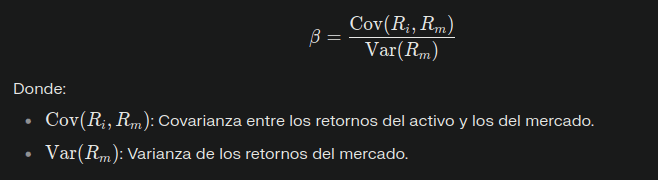
Interpretation
- β=1: The asset has the same volatility as the market.
- β>1: The asset is more volatile and riskier than the market.
- β<1: The asset is less volatile and therefore more defensive.
- β<0: The asset moves in the opposite direction to the market.
Code in Python
We are going to program a function that extends our class and calculates the Beta and Alpha values for the strategies.
    def calculate_greeks(self, benchmark_returns=None):
        import numpy as np

        if not self.trades:
            return 0, 0

        if isinstance(self.trades, list):
            trades_df = pd.DataFrame(self.trades)
        else:
            trades_df = self.trades

        strategy_returns = trades_df['Points'].values

        if benchmark_returns is None:
            if hasattr(self, 'df') and 'Close' in self.df.columns:

                benchmark_returns = self.df['Close'].diff().dropna().values

                if len(benchmark_returns) != len(strategy_returns):
                    benchmark_returns = benchmark_returns[:len(strategy_returns)]

                    if len(benchmark_returns) != len(strategy_returns):
                        return 0, 0

        if benchmark_returns is None or len(benchmark_returns) != len(strategy_returns):
            return 0, 0

        if not isinstance(benchmark_returns, np.ndarray):
            benchmark_returns = np.array(benchmark_returns)

        covariance = np.cov(strategy_returns, benchmark_returns)[0, 1]
        variance = np.var(benchmark_returns)
        beta = covariance / variance if variance != 0 else 0

        avg_strategy = np.mean(strategy_returns)
        avg_benchmark = np.mean(benchmark_returns)
        alpha = avg_strategy - (beta * avg_benchmark)

return beta, alpha- If there are no recorded trades (
self.tradesis empty), it returns(0, 0)as Beta and Alpha. - Converts the trades (
self.trades) into aDataFrameif it is a list. - Extracts the strategy returns from the
'Points'column. - If no benchmark returns (
benchmark_returns) are provided, it calculates returns based on closing prices ('Close') of the original asset. - Aligns the length of the benchmark returns with those of the strategy; if they don't match, it returns
(0, 0). - Calculates Beta
- If the benchmark variance is zero (no market movements), Beta is set to
0. - Calculates Alpha
- Returns the calculated Beta and Alpha values as a tuple
(beta, alpha).
Max Drawdown (MDD)
Max Drawdown corresponds to the maximum historical loss the strategy has suffered in the past. Since we are working with futures, we calculate it as maximum loss points, instead of percentages, and it serves to give us an approximation of how far the strategy went in the past toward a maximum loss.
So we extend our class with the calculations
    def calculate_mdd(self, trades=None):
        import numpy as np

        if trades is None:
            if not self.trades:
                return 0
            trades = pd.DataFrame(self.trades) if isinstance(self.trades, list) else self.trades

        if len(trades) == 0:
            return 0

        equity_curve = trades['Points'].cumsum()

        running_max = np.maximum.accumulate(equity_curve)

        drawdowns = (equity_curve - running_max)

        if np.max(running_max) == 0:
            return 0

        max_drawdown = np.min(drawdowns)

return abs(max_drawdown)- If no trades (
trades) are provided, it uses the trades recorded in the instance (self.trades). - Converts the trades into a
DataFrameif they are a list. - If there are no trades, it returns
0as the MDD. - Calculates the equity curve by accumulating the results of the trades (
Points) usingcumsum(). - Finds the cumulative maximums in the equity curve using
np.maximum.accumulate. - Calculates drawdowns as the difference between the equity curve and the cumulative maximums.
- If the cumulative maximum is zero (for example, if there are no gains or losses), it returns
0. - Finds the minimum value in the drawdowns (greatest cumulative loss).
- Returns the absolute value of the maximum drawdown as the result (positive convention).
Sharpe Ratio
The Sharpe Ratio, developed by William F. Sharpe, is a financial metric that measures the risk-adjusted return of an investment. Its objective is to determine whether an investment's returns are due to smart decisions or simply to assuming greater risk. It is widely used to compare investments and evaluate the quality of performance relative to the risk assumed.
Formula
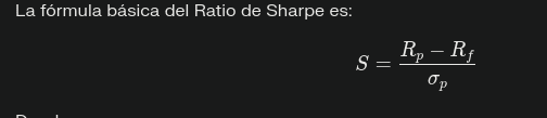
Where:
- Rp: Average return of the investment or portfolio.
- Rf: Return of the risk-free asset (such as Treasury bonds).
- σp: Standard deviation of the investment's returns (volatility).
Advantages and Limitations
Advantages
- Allows comparing investments with different risk levels.
- Adjusts returns based on risk, facilitating more objective analysis.
- Useful for evaluating portfolio managers or trading strategies.
Limitations
- Assumes that returns have a normal distribution, which is not always true.
- Does not distinguish between positive volatility (gains) and negative volatility (losses), which can penalize strategies with high positive variability.
    def calculate_sharpe_ratio(self, trades=None, risk_free_rate=0, periods_per_year=252):
        if trades is None:
            if not self.trades:
                return 0
            trades = pd.DataFrame(self.trades) if isinstance(self.trades, list) else self.trades

        if len(trades) == 0:
            return 0

        returns_mean = trades['Points'].mean()
        returns_std = trades['Points'].std()

        if returns_std == 0:
            return 0

        sharpe = (returns_mean - risk_free_rate) / returns_std
        annualized_sharpe = sharpe * np.sqrt(periods_per_year)
        return annualized_sharpe
Summary - Create statistics on the TradeHistory
Once we have programmed all the statistics functions, we are going to program a function that creates a 'summary' over our tradehistory. Extremely useful information, for when we launch our broad-spectrum optimization, to be able to locate the time zones with some kind of edge, or even create our ratios derived from the currently calculated ratios.
    def get_summary(self, benchmark_returns=None, confidence_level=0.95,):

        if not self.trades:
            return {"message": "No trades found"}

        trades_df = pd.DataFrame(self.trades)

        winning_trades = trades_df[trades_df['Points'] > 0]
        losing_trades = trades_df[trades_df['Points'] < 0]

        # Calcular SQN
        sqn_value = self.calculate_sqn(trades_df)

        # Calcular VaR y CVaR
        var, cvar = self.calculate_var_cvar(confidence_level)

        # Calcular alpha y beta si hay benchmark
        beta, alpha = self.calculate_greeks(benchmark_returns)

        # calculate MDD
        mdd = self.calculate_mdd(trades_df)

        # Calcular Sharpe Ratio
        sharpe_ratio = self.calculate_sharpe_ratio(trades_df)
        # Calcular el Summary
        summary = {
            'total_trades': len(trades_df),
            'mdd': mdd,
            'winning_trades': len(winning_trades),
            'losing_trades': len(losing_trades),
            'win_rate': len(winning_trades) / len(trades_df) if len(trades_df) > 0 else 0,
            'avg_profit': trades_df['Points'].mean(),
            'total_profit': trades_df['Points'].sum(),
            'max_profit': trades_df['Points'].max(),
            'max_loss': trades_df['Points'].min(),
            'variance': np.var(trades_df['Points']),
            'profit_factor': abs(winning_trades['Points'].sum() / losing_trades['Points'].sum())
                           if len(losing_trades) > 0 and losing_trades['Points'].sum() != 0 else float('inf'),
            'sharpe': sharpe_ratio,
            'sqn': sqn_value,
            'VaR': var,
            'CVaR': cvar,
            'beta': beta,
            'alpha': alpha
        }

        return summary
This code defines a method called get_summary that generates a detailed statistical summary of the operations performed by a trading strategy. It combines several key metrics to evaluate the performance, risk, and quality of the strategy.
- If there are no trades (
self.tradesis empty), it returns a message indicating that no trades were found. - Converts the trades (
self.trades) into aDataFrameto facilitate calculations. - Separates winning trades (
winning_trades) and losing trades (losing_trades) based on the'Points'column. - SQN: Calls the
calculate_sqnmethod to calculate the System Quality Number. - VaR and CVaR: Calls the
calculate_var_cvarmethod to calculate Value at Risk and Conditional Value at Risk with a specified confidence level. - Alpha and Beta: Calls the
calculate_greeksmethod if benchmark returns are provided. - MDD: Calls the
calculate_mddmethod to calculate the Maximum Drawdown. - Sharpe Ratio: Calls the
calculate_sharpe_ratiomethod to measure risk-adjusted return. - Total number of trades, winners and losers.
- Win rate: Percentage of winning trades.
- Average, total, maximum profit and maximum loss.
- Variance of the results.
- Profit Factor: Ratio between total gains and total losses (if there are losses).
- Compiles all calculated metrics in a dictionary called
summary. - Returns the dictionary with all key statistics.
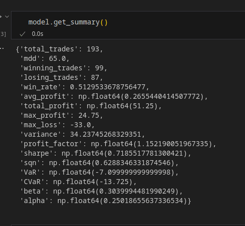
All metrics included in the summary
| Metric | Description |
|---|---|
total_trades |
Total number of trades made. |
mdd |
Maximum Drawdown: Greatest cumulative loss from a peak to a valley in the equity curve. |
winning_trades |
Number of winning trades. |
losing_trades |
Number of losing trades. |
win_rate |
Percentage of winning trades over the total. |
avg_profit |
Average profit per trade. |
total_profit |
Total accumulated profit. |
max_profit |
Maximum profit obtained in a single trade. |
max_loss |
Maximum loss suffered in a single trade. |
variance |
Variance of the results (measure of dispersion). |
profit_factor |
Ratio between total gains and total losses (efficiency indicator). |
sharpe |
Sharpe Ratio: Risk-adjusted return. |
sqn |
System Quality Number: System quality based on risk and performance. |
VaR |
Value at Risk: Maximum expected loss with a given confidence level. |
CVaR |
Conditional Value at Risk: Average loss beyond VaR (extreme risk). |
beta |
Sensitivity of the system to market movements (benchmark). |
alpha |
Additional performance generated by the strategy adjusted for systematic risk (benchmark). |
Implementation of what has been programmed so far
The first step is to load the libraries, in this case pandas to load the pickle of the data, and our IntradaySeasonalBacktester from the notebook

Subsequently, we will load our pickle into a dataframe, in this case it is the ES future preprocessed as explained in article 1, but it can be from any other asset.
We create an instance of our IntradaySeasonalBacktester called model, we pass our preprocessed data dataframe as an argument, and I have put some random parameters for entry day of the week, entry hour, entry minute, and bars inside.
Subsequently we run the backtest with the run_backtest() method to generate the TradeHistory of the strategy.
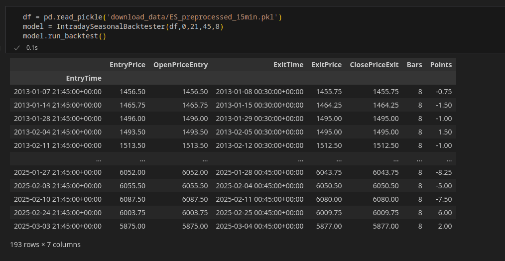
And now we are going to request a summary of the trades of the strategy we just ran, by calling the get_summary() function, which will call all the advanced statistics we have calculated, as well as other simpler ones that we calculate directly with pandas and numpy. Obtaining the data necessary for an evaluation of the strategy.
Links of Interest
 Full Bio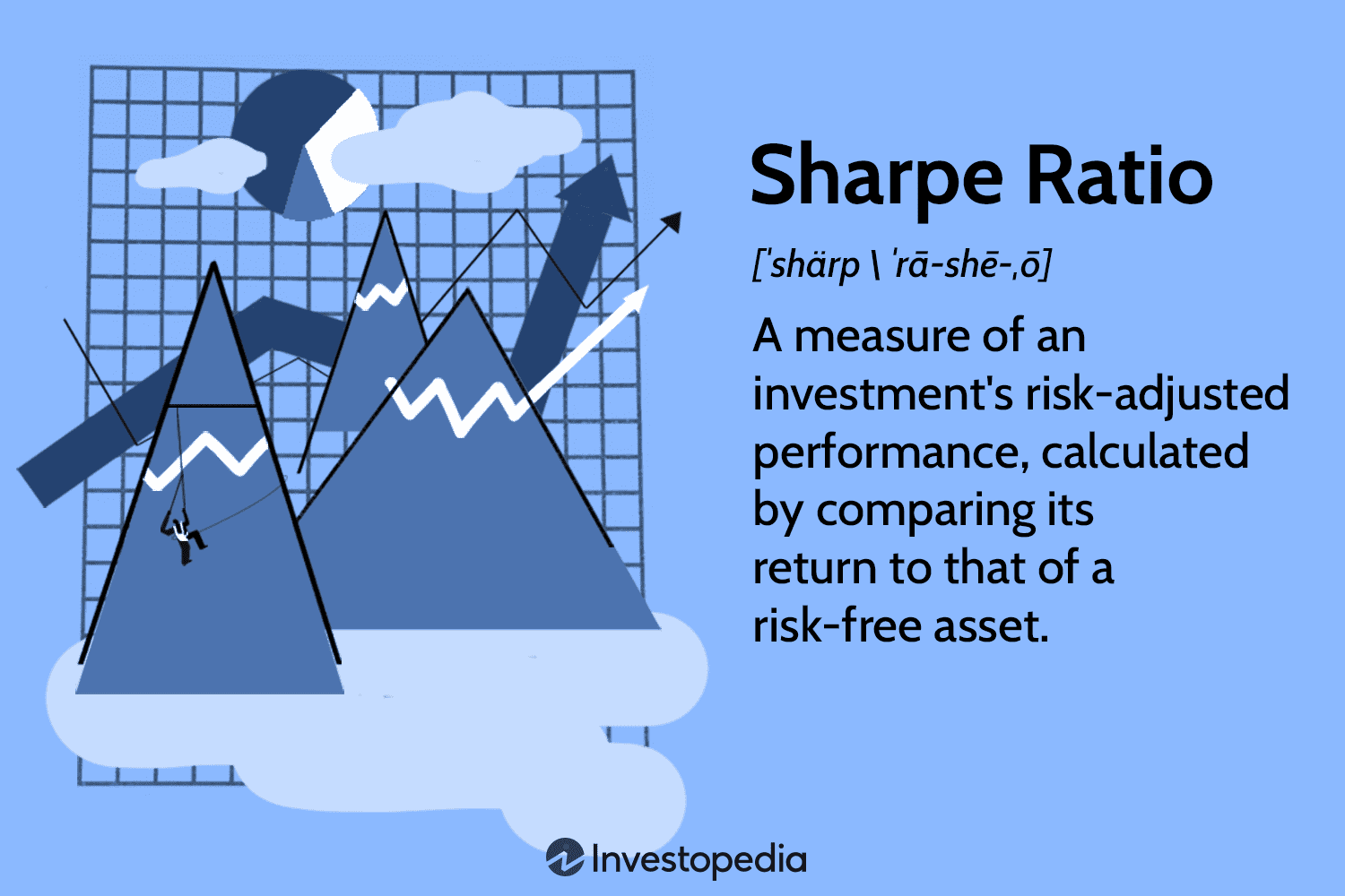
 Full Bio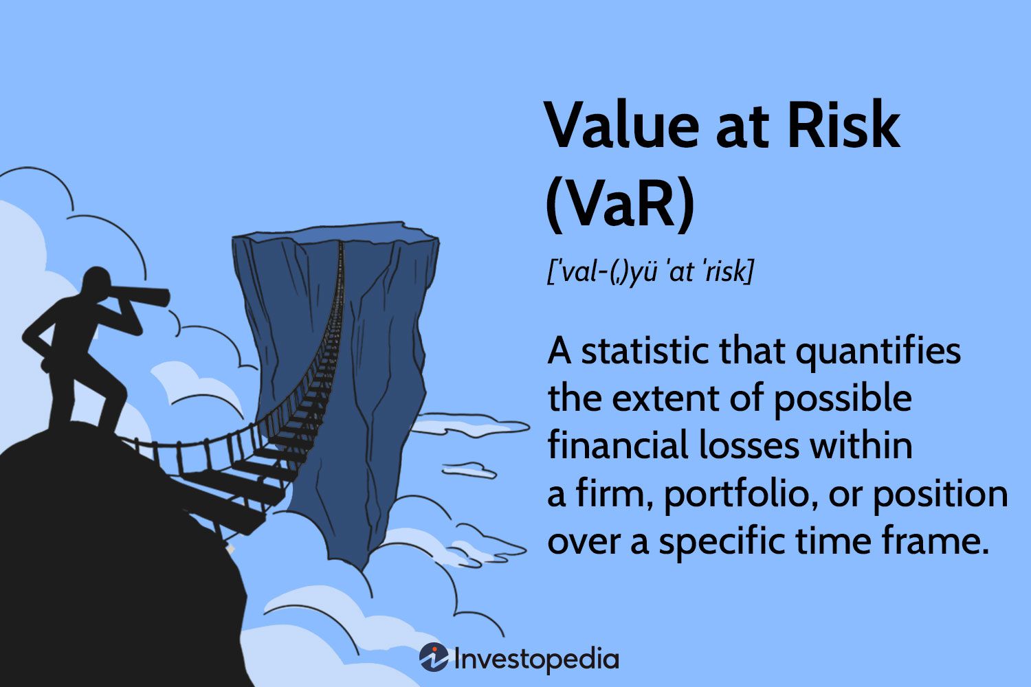
 Full Bio
 rcanessa
Coming Soon
In the next article, we will create a broad-spectrum analyzer that investigates all time bands of the asset, searching for intraday seasonal patterns. Using all the previously programmed methods and returning a dataframe with the parameters used and the statistics of that combination, to subsequently run an analysis.
For any questions, do not hesitate to contact me by email at jcx[a]quantarmy.com
Greetings, Jesús.