
In the first part of this series, we defined what we are looking for, what intraday seasonality is, its causes and its consequences. In this new article, we will build the foundation of our entire study, the backtester that will verify the hypotheses about the strategies, generating the buy and sell operations necessary to validate whether an advantage really exists or not.
This article aims to be an introduction to seasonal backtesting; the model can be widely improved, but its basic functionality is robust enough and easy to understand to be able to extend it later with more functionality.
Other installments of the series
 Jesús Cuesta
 Jesús Cuesta
Action Plan
In the first article, we preprocessed the data for later use. The plan for this article is, with that preprocessed data, to be able to backtest seasonal models in a simple way. No stops, no take profits, no commissions, just a repeated and sustained entry throughout the history meeting fixed requirements and subsequently analyzing the results.
To do this, we will create a class where we will expand all the necessary methods; we will program the backtester using pandas masks, since there is no point in reinventing the wheel. It could be done with libraries like backtrader or backtesting.py, but really, it's easier for me to build it from scratch. So let's get to it
Creating the class for backtesting intraday seasonal models in Python.
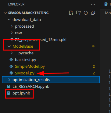
Inside the ModelBase folder, we will create the class inside the SModel.py file. Also outside the folder, we will create a notebook called ppt.ipynb where we will run the algorithm, leaving a structure like this, ignoring the rest of the files for now.
IntradaySeasonalBacktester Class
The first thing we will do is import the libraries we will use. In this case pandas and numpy. For now we don't need more libraries.
The way we have to define the class is through
class IntradaySeasonalBacktester:The next step is to assign it some arguments, which will be the parameters of our strategy; to do this we will do it inside the __ init __ function which will be:
- df: through this parameter, we will include the previously preprocessed dataframe
- entry_weekday: through this parameter we will tell it which day of the week it has to search for, where 0 is Monday and 6 is Sunday.
- entry_hour= through this parameter we will tell it at what hour it will enter
- entry_minute= through this parameter we will tell it at what exact minute it will enter
- bars_to_exit = through this parameter we will tell it how many candles it will be inside the operation; since we preprocessed in 15-minute candles, 4 candles equals one hour.
Leaving the __ init __ of the function as follows
class IntradaySeasonalBacktester:

    def __init__(self, df, entry_weekday=None, entry_hour=None,
    entry_minute=None,bars_to_exit=1):
        self.df = df.copy()
        self.entry_weekday = entry_weekday
        self.entry_hour = entry_hour
        self.entry_minute = entry_minute
        self.bars_to_exit = bars_to_exit
        self.trades = []
In the IntradaySeasonalBacktester code, self is simply a reference to the specific instance of the object we are creating. It is a fundamental concept in object-oriented programming in Python.
self allows each instance of our backtester to:
- Maintain its own data (such as the price dataframe)
- Store its own parameters (such as entry times)
- Record its own results (in the
self.tradeslist)
When we write self.df = df.copy() or self.entry_hour = entry_hour, we are creating unique attributes for that particular instance of the backtester.
Without self, it would be impossible to run multiple tests with different parameters simultaneously, since there would be no way to distinguish which instance each variable belongs to.
Finding the intraday seasonal entries
Once the init function is finished, we will create a function that, from the introduced arguments, allows us to find the entries within the dataframe with the asset's data. To do this, we will use pandas masks, for code simplicity and efficiency, so that the function can later be called from the backtester.
Leaving the function as:
    def find_entries(self):
        entries = (self.df['weekday'] == self.entry_weekday) & \
                (self.df['hour'] == self.entry_hour) & \
                (self.df['minute'] == self.entry_minute)
In this way we assign what the entries are, when in our dataframe the weekday field matches the one we requested in the init function, and the same for the entry hour and exit hour.
Through this function we have defined the entries, accelerating and simplifying the backtesting process to just a function within the class.
So far, everything coded looks like this:
class IntradaySeasonalBacktester:
    def __init__(self, df, entry_weekday=None,
    entry_hour=None, entry_minute=None,
                 bars_to_exit=1):
        self.df = df.copy()
        self.entry_weekday = entry_weekday
        self.entry_hour = entry_hour
        self.entry_minute = entry_minute
        self.bars_to_exit = bars_to_exit
        self.trades = []

    def find_entries(self):
        entries = (self.df['weekday'] == self.entry_weekday) & \
                (self.df['hour'] == self.entry_hour) & \
                (self.df['minute'] == self.entry_minute)

        return entries
The result we get when making a call to the find_entries function and verifying its operation is
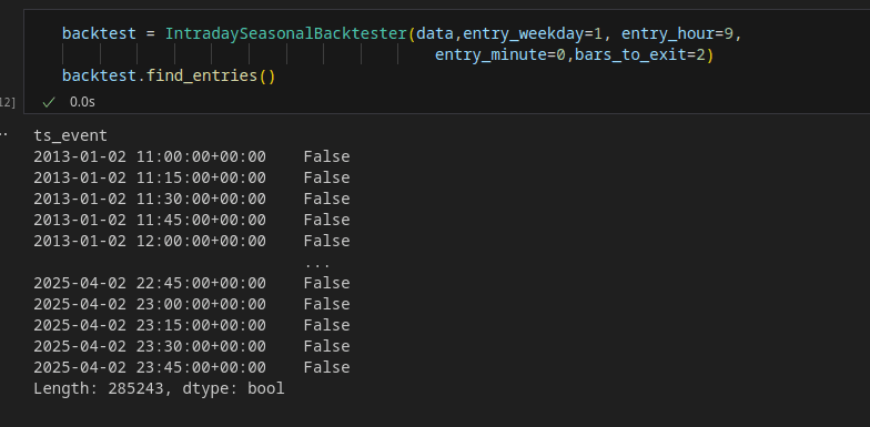
As we can see, it responds with True or False depending on whether the row meets the requirements or not. Subsequently, with the use of pandas, we will be able to filter among the data those that are entries to locate them in an agile way, and be able to process the backtest.
Backtesting Function
Once we have clear the entry conditions, the next step is to create a function within the class that executes the backtest in a simple and agile way. And let's get to it
First steps of backtesting
The first steps within our backtesting structure will be:
- Find the entry points
- Work with numeric positions resetting the datetime indices
- Get the name of the first column to work with it later when jumping candles, since we come from a dataframe without an index to speed up the process
def run_backtest(self):
        # Encontrar los puntos de entrada
        entries = self.find_entries()
        entry_timestamps = self.df[entries].index

        # Reset index para trabajar con posiciones numéricas
        df_reset = self.df.reset_index()

        # Coje el nombre de la primera columna, para trabajar con fechas
        index_column_name = df_reset.columns[0]
With this code, we easily identify the entries, and store the indices (which have not yet been reset, keeping the dates saved for reuse in the future, when a entry point needs to be found.
We create a dataframe with the reset index, and get the name of the column that was formerly the index, because that is where the current temporal qualities are stored, such as the day and hour when the records occur.
Date Processing
Once we have identified the dates where the entries will occur, we will process them, performing the following steps
- We iterate through the entries
- We find the position in the df without index
- We verify that we can close the operation
- We save the entry data
- We save the exit data
- We calculate the variation of the operation
- We save the operation within the trade register
        for entry_timestamp in entry_timestamps:
            entry_position = df_reset[df_reset[index_column_name] == entry_timestamp].index[0]

            if entry_position + self.bars_to_exit >= len(df_reset):
                continue

            entry_row = df_reset.iloc[entry_position]
            entry_price = entry_row['Open'] # Entramos en Apertura

            exit_position = entry_position + self.bars_to_exit
            exit_row = df_reset.iloc[exit_position]
            exit_price = exit_row['Close']
            exit_timestamp = exit_row[index_column_name]

            points = exit_price - entry_price

            self.trades.append({
                'EntryTime': entry_timestamp,
                'EntryPrice': entry_price,
                'OpenPriceEntry': entry_row['Open'],
                'ExitTime': exit_timestamp,
                'ExitPrice': exit_price,
                'ClosePriceExit': exit_row['Close'],
                'Bars': self.bars_to_exit,
                'Points': points
            })
through this simple and agile code, we have scanned all days where there is an entry, we verify if we can close the operation through
            if entry_position + self.bars_to_exit >= len(df_reset):
                continue
And we start capturing the necessary values to be able to generate the operations, we even calculate the variation in points of the operation. Since we are working with futures, we use basic point accounting
            entry_row = df_reset.iloc[entry_position]
            entry_price = entry_row['Open'] # Entramos en Apertura
            exit_position = entry_position + self.bars_to_exit
            exit_row = df_reset.iloc[exit_position]
            exit_price = exit_row['Close']
            exit_timestamp = exit_row[index_column_name]
            points = exit_price - entry_price
TradeHistory
The dataframe that will provide information about the model we just simulated, we call TradeHistory. The TradeHistory shows all cases where an entry has occurred and everything calculated, in an ordered dataframe, which will later be the raw material for calculating relevant statistics to analyze the viability of the strategy.
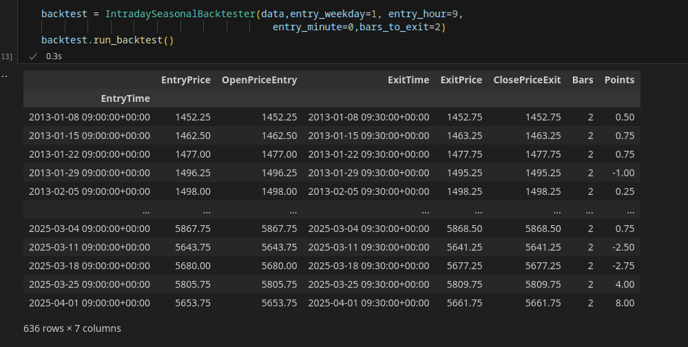
When running the backtest, it directly returns the TradeHistory, with the following parameters
- EntryTime: Hour and Day when the entry is made
- EntryPrice: Theoretical Entry Price
- OpenPriceEntry: Open price of the entry candle (to simulate slippage in the future between OpenPriceEntry and EntryPrice)
- ExitTime Hour and Day of Exit
- ExitPrice: Theoretical Exit Price
- CloseExitPrice: Close price of the exit candle
- Bars: Number of candles within the operation
- Points: Variation in points between exit_price and entry_price. Since these are futures, this is the profit; to convert it to dollars, you would have to multiply it by the dollar per point of the contract specifications.
How to use it from the notebook
The first step, respecting the file structure, is to load the libraries

Subsequently we will load the preprocessed data, in my case the ES future data

The next step is to launch an instance of IntradaySeasonalBacktester on the data dataframe (which contains ES future data) entering on day 1 (Tuesday) at 9:00 and exiting after two bars, that is at 9:30

Once we launch the instance we see that it has been executed correctly

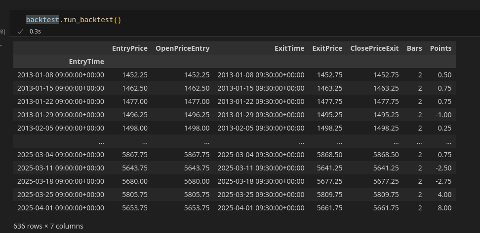
And once with the dataframe loaded and the necessary arguments, we can launch the backtest as follows, returning the TradeHistory
Conclusions
In this installment, we have created the first backtesting model, which already lets us test hypotheses in a simple way for intraday seasonal patterns. This model is the foundation of everything, which in the following installments we will expand in functionality and purpose. But as an introduction to intraday seasonal backtesting in Python, it is more than enough.
Next Article
In the next article, we will process the operations to extract the most relevant statistics, run some randomness test, and start looking for hints of alpha among all the data. And we will settle all the concepts so that in a later installment we can begin a broad-spectrum optimization, searching across the entire operational field for the relevant zones where seasonal patterns occur, which can serve as a starting point for future research toward a fully functional and tradable model.
See you in the next installment, and any questions jcx[a]quantarmy.com