
Do you want to learn quantitative trading and automate your strategies? This python trading course is the definitive guide to start programming, analyzing, and optimizing trading systems with Python, the most widely used tool by traders and quants worldwide.
This article was updated in April 2025 to adapt the code to the latest updates of the libraries in use.
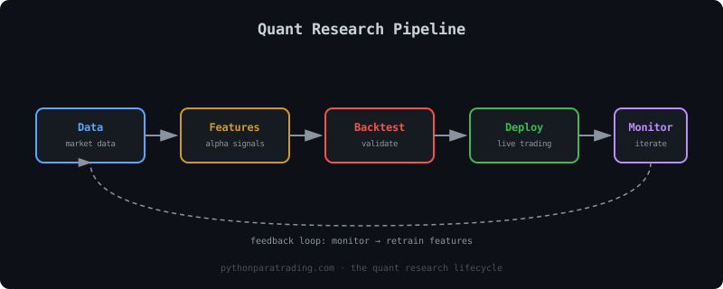
Why learn trading with Python?
Trading in financial markets is constantly evolving. Python allows you to:
- Automate strategies and analysis.
- Access historical and real-time data.
- Perform backtesting and system optimization.
- Visualize results and risk metrics.
Mastering Python is key for any modern trader.
Essential libraries for trading in Python
For this python trading course we will use:
- Pandas: tabular data analysis and manipulation.
- Numpy: numerical calculations and matrix operations.
- Matplotlib: data visualization and plotting.
- yfinance: downloading financial data from Yahoo Finance.
- itertools: efficient generation of parameter combinations.
- quantstats: performance and risk metrics.
- warnings: warning management in Python.
import pandas as pd
import numpy as np
import yfinance as yf
import matplotlib.pyplot as plt
from itertools import product
import quantstats as qs
import warnings

%matplotlib inline
warnings.filterwarnings("ignore")
Data download and initial variables
We define the moving average parameters and download the historical data of the SPY ETF (S&P 500):
media_1 = 20
media_2 = 3 * media_1
df = yf.download('SPY', interval='1d')
df.columns = df.columns.droplevel(1)
df = df['2023':]
Using yf.download, we download the daily SPY data. By using df.columns = df.columns.droplevel(1), we remove the unnecessary multi-index, and we reduce the history to start in 2023 for the sole purpose of better visualizing the signals generated by the algorithm.
Calculation and visualization of moving averages
We calculate the moving averages on the adjusted close price:
df['Avg_1'] = df['Adj Close'].rolling(media_1).mean()
df['Avg_2'] = df['Adj Close'].rolling(media_2).mean()
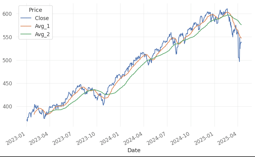
We visualize the price and the moving averages:
df[['Close', 'Avg_1', 'Avg_2']].plot()The result would look something like this.
Generating and visualizing trading signals
We create entry and exit signals based on moving average crossovers. We will use the where function from the numpy library. It evaluates a condition, and if positive, assigns the value 1 or True, and otherwise assigns the value 0 or False. Generating signals only when average 1 or avg_1 is below average 2 or avg_2.
The .shift(1) command evaluates the immediately preceding candle to act on the current candle. Otherwise, we would be filtering future information, generating overfit in the strategy and unrealistic returns.
df['In_Trade'] = np.where(df['Avg_1'].shift(1) < df['Avg_2'].shift(1), 1, 0)
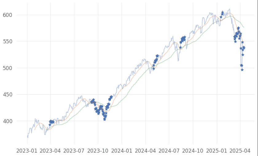
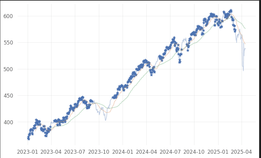
We visualize the entry and exit signals on the chart:
# Entry signals
idx_open = df.loc[df["In_Trade"] == 1].index
plt.scatter(idx_open, df.loc[idx_open]["Close"], marker="*")
plt.plot(df["Close"].index, df["Close"], alpha=0.35)
plt.plot(df["Close"].index, df["Avg_1"], alpha=0.35)
plt.plot(df["Close"].index, df["Avg_2"], alpha=0.35)
plt.show()

# Exit signals
idx_open = df.loc[df["In_Trade"] == 0].index
plt.scatter(idx_open, df.loc[idx_open]["Close"], marker="*")
plt.plot(df["Close"].index, df["Close"], alpha=0.35)
plt.plot(df["Close"].index, df["Avg_1"], alpha=0.35)
plt.plot(df["Close"].index, df["Avg_2"], alpha=0.35)
plt.show()
The entry chart would look something like this:
And the exit chart would look something like this:
Profitability and drawdown analysis
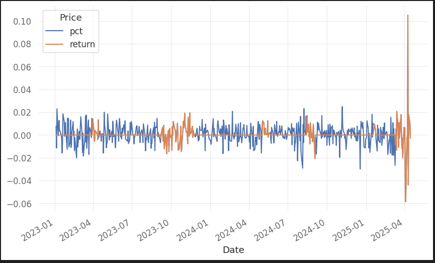
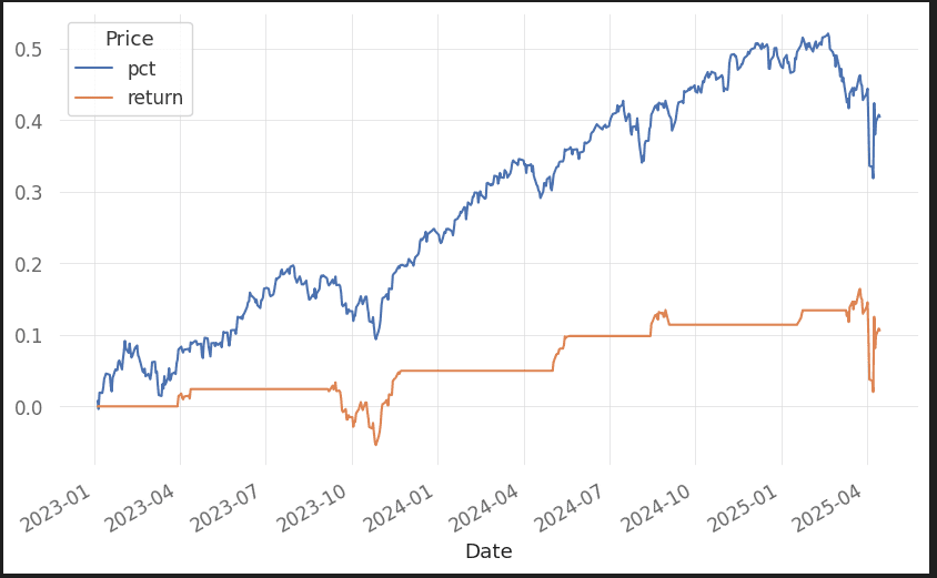
We calculate the daily return and the strategy return:
df["pct"] = df["Close"].pct_change()
df["return"] = df["pct"] * df["In_Trade"].shift(1)
df[['pct', 'return']].plot()
df[['pct', 'return']].cumsum().plot()
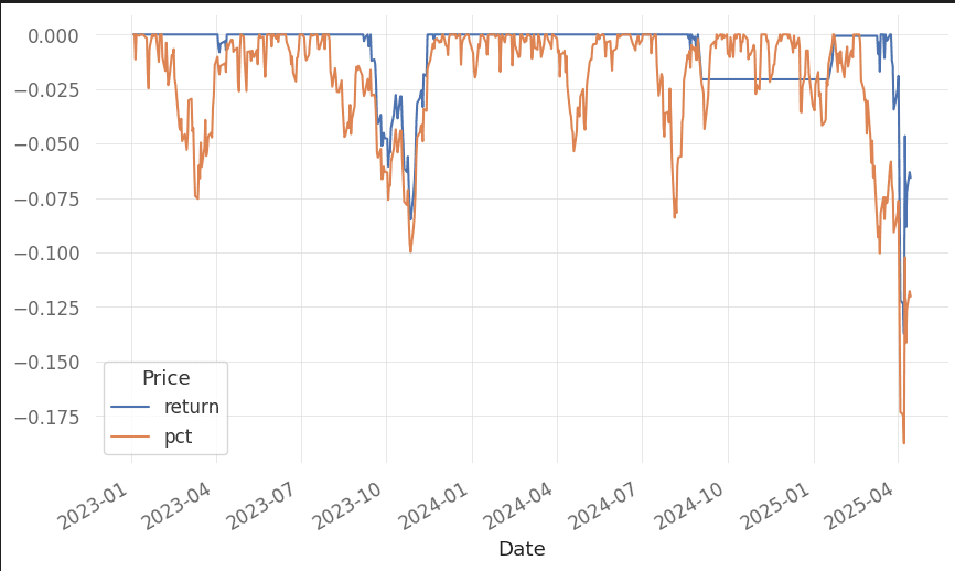
We visualize the strategy drawdown:
qs.stats.to_drawdown_series(df[['return', 'pct']]).plot()
The percentage variation would look like this:
And the sum of returns would look like this:
Trading system optimization
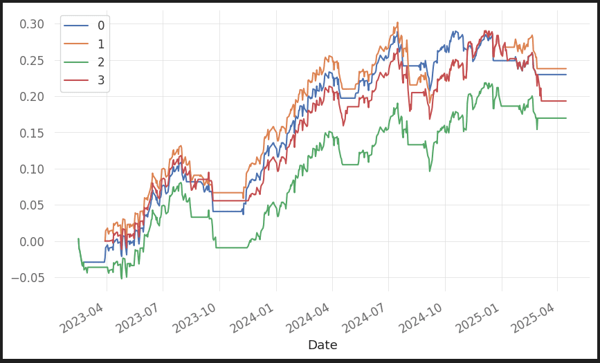
We test different combinations of moving averages to find the most profitable one:
rapido = [5, 15]
lento = [30, 60]
resultados = []
eqs = []
combinaciones = list(product(rapido, lento))
for media_rapida, media_lenta in product(rapido, lento):
    temp = pd.DataFrame()
    temp['Avg_1'] = df['Close'].rolling(media_rapida).mean()
    temp['Avg_2'] = df['Close'].rolling(media_lenta).mean()
    temp['pct'] = df['Close'].pct_change()
    temp.loc[(temp["Avg_1"].shift(1) > temp["Avg_2"].shift(1)), "In_Trade"] = 1
    temp.loc[(temp["Avg_1"].shift(1) < temp["Avg_2"].shift(1)), "In_Trade"] = 0
    ret_c = ((temp['In_Trade']) * (temp['pct'])).cumsum().dropna()
    ret = ((temp['In_Trade']) * (temp['pct']))
    greeks = qs.stats.greeks(ret, temp['pct'].dropna())
    sharpe = qs.stats.sharpe(ret)
    mdd = qs.stats.max_drawdown(ret)
    dom = len(temp[temp['In_Trade'] == 1]) / len(temp.index)
    var = qs.stats.value_at_risk(ret, 1) * 100
    resultados.append({'media_1': media_rapida, 'media_2': media_lenta, 'ret': ret_c[-1],
                      'beta': greeks[0], 'alpha': greeks[1], 'sharpe': sharpe, 'max_dd': mdd, 'on_market': dom, 'var': var})
    eqs.append(ret)
pd.DataFrame(resultados)
This code block performs a systematic optimization of the moving average crossover strategy by testing all possible combinations between various fast and slow moving average periods. For each combination, the fast and slow moving averages are calculated on the adjusted close price, entry and exit signals are generated, and both the daily and cumulative return of the strategy are calculated. Additionally, key performance and risk metrics are obtained, such as alpha, beta, Sharpe ratio, maximum drawdown, time in market percentage, and VaR, which are stored in a results list along with the daily returns of each combination.
Once finished, a DataFrame is built with all the results, making it easy to compare the performance of each moving average configuration. This automated process makes it easy to identify which parameters offer the best historical results and is fundamental for developing robust and quantitative trading systems.
The result it gives us is:

Visualization of all optimizations:
pd.DataFrame(eqs).transpose().cumsum().plot()
Key evaluation metrics:
- Alpha: risk-adjusted return relative to the market.
- Beta: sensitivity of the strategy relative to the market.
- Sharpe: ratio between excess return and volatility.
- Max Drawdown: maximum drop from a peak.
- Time on Market: proportion of time in the market.
- Value at Risk (VaR): maximum expected loss under a confidence level.
Frequently asked questions
Who is this python trading course for?
- Beginners in trading and programming.
- Traders who want to automate strategies.
- Quantitative and financial analysts.
Do I need prior Python experience?
- It's not essential, but it helps. The course is designed so you can follow it even if you're new to Python.
What are the advantages of using Python for trading?
- It's free, versatile, and has a huge community.
- It allows automating analysis, backtesting, and order execution.
- It's the standard in quantitative trading and financial analysis.
Summary and additional resources
This python trading course has shown you how to download data, calculate moving averages, generate signals, analyze results, and optimize your trading system. Mastering these tools will allow you to create and improve your own algorithmic trading strategies.
Keep learning:
Ready to take your trading to the next level?
Start your own python trading course now and automate your strategies.
If you want to access the complete and updated code, as well as other resources for members, we recommend signing up.
Any questions, contact me at jcx[a]quantarmy.com
Best regards, and see you next time!