

Quantitative Models, Algorithmic Execution, and Quantitative Trading
In this article we will discuss quantitative models in trading. We will explore different quantitative trading models and how they are executed through algorithms.
import numpy as np

# Kelly Criterion: optimal position sizing
def kelly_fraction(mu, sigma, rf=0.0):
    """f* = (mu - rf) / sigma^2"""
    return (mu - rf) / (sigma ** 2)

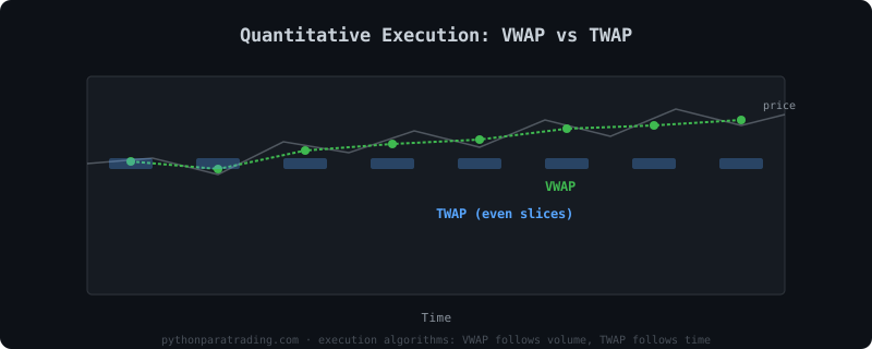
# VWAP execution: slice order by volume profile
def vwap_schedule(total_shares, volume_profile):
    """Split order according to historical volume curve."""
    weights = volume_profile / volume_profile.sum()
    return (total_shares * weights).astype(int)

# TWAP execution: equal time slices
def twap_schedule(total_shares, n_slices):
    """Split order into equal time intervals."""
    return np.full(n_slices, total_shares // n_slices)
To differentiate between these two concepts, we define them as:
- Algorithmic execution algorithms: A logical sequence of instructions, designed for a specific task (a program dedicated to executing pre-established signals).
- Quantitative models: Models are frameworks that enable us to extract alpha from the market (styles, strategy types, operational frameworks).
We can classify quantitative models into different investment styles. These quantitative models are combinations of factors that allow us to exploit a window of alpha exposure through modeling and calibration processes.
On the other hand, algorithmic execution algorithms are responsible for controlling assets in real time and managing the inventory of positions and capital based on the signals generated by the model. Colloquially referred to as algorithmic execution.
History of Algorithmic Trading
Algorithmic trading is a relatively recent phenomenon. In the 1990s, more than 50% of transactions took place on trading floors, physical environments where securities were exchanged amid shouts. The other 50% was already carried out electronically, with no need to be physically present to execute an order. At that time, approximately 2-3% corresponded to algorithmic executions, that is, signal generation models and automatic execution.
In the 2000s, with the popularization of derivative products, the major market participants began hiring mathematicians, physicists, and programmers to join their teams. This gave rise to an ecosystem of tools and protocols that were only available to members of those banks and investment funds.
Today, that technological gap between banks and the rest of participants has been reduced thanks to the spread of knowledge and the growth of projects offering specialized tools, methods, and procedures.
Practically anyone with around 5,000 euros to invest in a server can have a setup similar to the one used in the last year of operations at Lehman Brothers.
Initially, algorithms were used to calculate the price of options and to estimate the impact on risk in banks' balance sheets. That is, to assign a real value to the strike price of an option and to exploit arbitrage opportunities between the estimated price and the real price. Or to gain better visibility into the current risk of the portfolio, for future decision-making. Later, their use spread to all financial products.
Today, even assets that are traditionally traded over the counter, such as debt issuance and placement operations, have been completely digitalized. There are even models that generate alpha (additional return) in these scenarios.
The application of computing and technology to the financial sector has brought about a great advance and has revolutionized everything from payment methods to asset classes and any other variable needed in day-to-day operations, creating new ways to invest.
What Is a Trading Algorithm?
Algorithmic execution algorithms are logical sequences that follow rules pre-established by quantitative models. Their main function is to bring to production—that is, to the real market environment—the signals from the quantitative models. These algorithmic execution processes handle everything from orders, collateral, and risks, among other aspects. Efficiency in trading algorithms translates into faster execution and a lower probability of facing adverse situations when taking positions in the market.
Trading algorithms can encompass various functionalities depending on how far their creator extends them. They can include alert systems, risk management, inventory management, real-time sentiment analysis, among others.
In this first part, we will focus on the types of algorithmic execution. When bringing a model to production, it is important to understand its scope of operation and objectives. It makes no sense to program an orderbook reading system if operations are carried out on a daily timeframe, for example. The first step is to understand the needs and evaluate the optimal way to implement them.
The three most relevant factors for algorithm design would be:
- Understand the execution opportunities. It makes no sense to build an optimized deployment for a quantitative model based on sector rotation with quarterly rebalancing.
- Understand the execution context: Study the order book from top to bottom. Understand all its characteristics in order to generate an attack plan afterward. The ultra-simplistic reduction that could be considered valid in certain scenarios consists of using market orders in assets with very high liquidity, assuming negligible slippage (price slippage from the moment an order is placed until it is executed). Given that these are often extremely liquid assets, the simplification of using market orders and assuming a small constant slippage is not an exact approximation of reality, but it is close to the impact that quantitative models could suffer when entering production.
- Clearly understand the flow of the algorithm's logic, and generate verification strategies. In real production environments, as in war, plans seem robust until they are executed in real markets. That is why we must try to minimize as many contingencies as possible, since each error usually has a negative impact on the returns of our strategy. Constant monitoring and supervision are fundamental parts of any algorithmic execution model.
We are going to classify 3 types of algorithms, the most used by retail traders. And I particularly classify them according to their operating windows.
- Time-based predisposition algorithms
- Dynamic operating algorithms
- Opportunistic operating algorithms
Time-based predisposition algorithms
These models are characterized by having a strong temporal component. They are algorithms that operate within specific time intervals. They detect small inefficiencies that occur at specific moments in the market due to various reasons and try to exploit those inefficiencies to extract alpha when certain conditions are met.
A clear example could be an algorithm that executes trades from market open until a certain nominal volume has accumulated. Or simply, being limited to operating within specific time ranges.
The advantage of these models lies in understanding the market context and adapting to specific operating conditions. Some institutions have highly advanced automation for this type of operations and generally do not try to hide their activity. Agricultural commodities markets are a common example worth investigating. In addition, specific moments such as market openings or closings, or data release hours, generate greater activity in contracts and greater price volatility, which can be a favorable scenario for extracting alpha.
Dynamic operating algorithms
Dynamic operating algorithms are those trading algorithms that do not have a specific time interval to operate, but can trade at any time while the asset is being quoted. These algorithms are constantly receiving price information and evaluating pre-established conditions to deploy an order and execute it in the shortest possible time.
For example, these algorithms can modulate the size of trades based on current traded volume, or they can be specifically designed to operate under particular market conditions, such as having a more accessible threshold for executing orders during periods of rising volatility.
In retail trading, these algorithms are often used to buy when certain indicators, such as Bollinger Bands or others, deviate, and pricing systems that have proven profitable in historical tests are also included.
As a personal anecdote, I can say that 90% of the people who have shown me an algorithm have based their concepts on a combination of these two categories. For example, looking for deviations from the open through the first 30 minutes and, if none occur, using the price as a reference for the session close.
Opportunistic algorithms
These algorithms belong to one of my favorite categories. They are highly dynamic and opportunistic, as they only operate at key moments. Let me give an extreme but illustrative example. Imagine an algorithm programmed to buy the S&P 500 when it falls -3 sigmas.
This algorithm will be in a flat position (with no open trades) most of the time, until an unusually extreme market drop occurs, in this case of -3 sigmas. At that point, it will enter the market and remain there until a similar event occurs again.
These algorithms are based on Nassim Taleb's principle of asymmetric risk. One of his strategies consisted of hedging the tails of the British pound curve, assuming an annual loss of -3% in exchange for being protected (and multiplying returns to three digits) in the event of more extreme-than-usual events.
These algorithms seek to capture opportunities during moments of high volatility or unusual events, applying an asymmetric risk strategy that aims to benefit from exceptional market movements.
Trading Strategies
What Is a Trading Strategy?
A trading strategy is a quantitative model that establishes a set of rules to guide the signal generation flow in trading. These strategies provide a systematic view to generate signals and manage other variables based on pre-established methods. There are different types of quantitative models, from the simplest based on technical analysis and accounting or sentiment analysis, to the most important such as quantitative models. Later on, we will explore the concept of the alpha factor, which is closely related to quantitative models.
For a strategy to be profitable, it must meet certain criteria:
- Consistency: It is essential that returns exhibit consistency in their characteristics. This implies that the characteristics of out-of-sample returns must be aligned with the characteristics of the quantitative models evaluated during the backtest.
- Risk Management: It must use favorable asymmetry in risk-reward ratios. Martingales make no sense, nor do strategies that risk 100% to gain 1%.
- Evaluable: They must be evaluable, comparable, and replicable. Strategies based on subjective patterns such as personal feelings.
A trading strategy is a set of rules on how it should evaluate and ex
Quantitative Models
Within quantitative trading, or quant trading, there are many strategies, different modalities where signal generation comes from quantitative models. Each investment style has its particular characteristics, and this is a list of the most common styles. All these rules that characterize strategies are referred to as quantitative models. A fundamental part of algorithmic trading, as it dictates the signals that will later be crossed using algorithmic execution.
Trend Following
Quantitative models known as Trend Following models or trend followers are widely used quantitative models. The model's main source of alpha consists of the asset's own beta.
They seek the persistence of repeated patterns in directionality, assuming that if an asset has high autocorrelation, or any test that could determine with a certain margin of safety that it is a trending asset, in order to identify an entry point and acquire exposure to the supposed trend.
There are extremely simple quantitative models for this factor, such as a simple moving average crossover, up to more elaborate ones. But the fundamental essence is the same in both cases.
Mean Reversion
They assume that prices will eventually revert to their historical mean, or to a previous level, if the deviation has been very abrupt. Basically, the main objective is to expose this style of strategies against strategies with a strong mean reversion component.
Usually in highly traded assets, such as an American index, moments of panic generate noise in the price, exaggerating price movements and providing opportunities to gain exposure to the asset.
Momentum Strategies
Momentum strategies seek to profit from continuation movements in price. They typically use breakouts of n-deviation ranges to take positions, assuming the continuation of the trend.
The objective of these strategies is to try to capture the hottest assets, evaluating market exposure points with different estimators.
Arbitrage Oportunities
Arbitrage strategies are based on obtaining profit from price differences in the market. For example, an asset listed on two different markets at different prices. Buying the cheap one and selling the expensive one provides an immediate profit. These strategies require broad financial and technological knowledge, since it is one of the most exploited sectors by traditional banks. In addition, arbitrage opportunities are usually negligible and require large accounts to sustain this type of positions.
Event Driven
Event-driven strategies are opportunistic strategies that gain market exposure at moments of key events and try to profit from the price movements that those events cause.
Market Neutral
Market Neutral strategies are based on generating consistent returns by exploiting the relationship between different quantitative factors, which ultimately generate neutral exposure to market movements. Attempting to eliminate beta and maximize the strategy's alpha.
Many of these portfolios are constructed through long positions in undervalued assets and short positions in overvalued assets. Using the value factor philosophy. Seeking returns from the performance of the assets, while, according to theory, "market risk" is "minimized."
Relative Value
A classic fixed-income strategy, it is based on exploiting a misvaluation of derivative assets. Through bonds as such, swaps, or futures. The main purpose is to discover that a derivative is not properly valued relative to its underlying asset, and to create a position that balances that discovery. Usually these strategies monitor the yield curve, credit spreads, and any other estimator that facilitates the discovery of the inefficiency and favors profitability when there is a convergence of criteria between the two assets (i.e., they correct the misvaluation).
Statistical Arbitrage
Statistical arbitrage is a quantitative strategy that attempts to exploit short-term divergences between asset prices, analyzing their historical price and their relationship with different assets.
Statistical arbitrage involves quantitative models and complex mathematical procedures to identify and exploit opportunities. Their attack niche is usually high-frequency trading (HFT) markets.
Some examples of statistical arbitrage would be pairs trading, index arbitrage, or volatility arbitrage strategies.
Pairs Trading
It is a sub-strategy of the so-called market-neutral strategies. Since it involves two products. A long leg and a short leg. Highly correlated assets are usually used, and the main objective is to obtain returns from the overperformance of one of the two legs. Using statistical analysis to find the attack vectors and market correlation, among other things.
It is a strategy that can be used with all types of assets, but one of the most common is in futures, through so-called spreads or other types of structures.
Machine Learning Based
They use advanced artificial intelligence algorithms to analyze large datasets and develop quantitative models based on data science processes.
This subgroup involves a wide range of techniques and strategies, each with distinct characteristics, but to add complexity, they are often mistakenly grouped into a single set.
Machine learning is not a factor per se; machine learning can carry out processes and identify candidate assets for any factor. It is the tool used to find attack vectors or solve any other purpose, not an investment style per se.
Global Macro Strategies
These strategies obtain their returns from macroeconomic models. Based on trends and geopolitical events that occur daily.
Starting from the premise that large-scale movements have repercussions on all aspects of life, including asset valuation, investors seek to take strategic positions to anticipate changes in the prices of those assets. These investors, specialized in political events and in understanding economic growth, typically take both long and short positions in assets such as fixed income, currencies, and commodities, although they may also have some exposure to equity markets.
In general, these strategies are discretionary and depend largely on the subjective judgment of the manager and their ideology. Recently, the most successful macro funds have been using quantitative models to identify opportunities, especially from the analysis of large amounts of alternative data.
Volatility Strategies
Volatility trading is a strategy focused on taking advantage of changes in an asset's volatility. When we refer to volatility, we mean price volatility, or historical volatility. Traders use these strategies to acquire volatility of the underlying asset and to exploit those movements. The most classic volatility strategy is the options structure known as straddles and strangles.
In addition, another very common use of volatility strategies consists of modulating risk exposure through delta hedges on the underlying asset of the main position.
$$f^* = \frac{\mu - r}{\sigma^2}$$
$$S = \frac{\mathbb{E}[R_p - R_f]}{\sigma_p}$$
$$\text{VWAP} = \frac{\sum_{j} P_j \times V_j}{\sum_{j} V_j}$$
$$\text{TWAP} = \frac{1}{N}\sum_{j=1}^{N} P_j$$