Impact of Seasonal Factor on US Bonds

In this article, we will analyze the impact of the seasonal factor on US Treasury bond yields. Seasonality is a phenomenon that occurs in many financial time series, and bonds are no exception.

What is Seasonality?

Seasonality refers to patterns or tendencies that repeat at regular intervals in a time series. In the context of bonds, this can manifest as systematic variations in yields depending on the time of year, month, or day of the week.

Methodology

To analyze the impact of seasonality on US bonds, we will follow these steps:

1. Download historical yield data for US Treasury bonds
2. Calculate the average yield by month, day of week, and other time periods
3. Identify patterns and statistically significant seasonal effects
4. Backtest a strategy based on the identified patterns

Data Download

We will use the yfinance library to download US Treasury yield data:

import pandas as pd
import yfinance as yf
import matplotlib.pyplot as plt

# Download US Treasury yield data
tickers = ['^TNX', '^TYX', '^FVX']
data = yf.download(tickers, start='2000-01-01')['Adj Close']
data.columns = ['10Y', '30Y', '5Y']

$$\bar{R}_m = \frac{1}{N_m} \sum_{t \in m} R_t, \quad m = 1, \ldots, 12$$

$$t = \frac{\bar{R}_m - \mu_0}{s_m / \sqrt{N_m}}, \quad p = 2 \times P(T > |t|)$$

$$S = \frac{\mathbb{E}[R_p - R_f]}{\sigma_p}$$

Seasonal Analysis

Once we have the data, we can analyze the seasonal patterns:

# Monthly average yields
monthly_avg = data.groupby(data.index.month).mean()

# Day of week average yields
dow_avg = data.groupby(data.index.dayofweek).mean()

# Plot monthly seasonality
fig, ax = plt.subplots(figsize=(12, 6))
monthly_avg.plot(ax=ax)
ax.set_title('Average Yields by Month')
ax.set_xlabel('Month')
ax.set_ylabel('Yield (%)')
plt.show()

Results

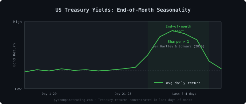
The results show that there are significant seasonal patterns in US Treasury yields. Some months tend to have higher yields than others, which can be exploited in trading strategies.

Seasonal Backtest

tickers = ['TLT', 'IEF', 'GOVT']
raw = yf.download(tickers)['Adj Close'].dropna()

# End-of-month signal
bt = pd.DataFrame()
last_day = raw.index.to_series().dt.daysinmonth
signal = raw.index.day >= (last_day - 5)
bt['signal'] = signal.astype(int)

pct = raw.pct_change()
bt['results'] = np.where(bt['signal'] == 1, pct.sum(axis=1), 0)
bt['cumulative'] = bt['results'].cumsum()
bt['cumulative'].plot(figsize=(14, 6), title='End-of-Month Seasonal Strategy')
plt.show()

Optimization by Lookback Days

def modelling_bonds(df, lookback_days):
    last_day = df.index.to_series().dt.daysinmonth
    signal = df.index.day >= (last_day - lookback_days)
    pct = df.pct_change()
    returns = np.where(signal, pct.sum(axis=1), 0)
    sharpe = returns.mean() / returns.std() * np.sqrt(252)
    return returns, sharpe

results = []
for x in range(0, 8):
    r, s = modelling_bonds(raw, x)
    results.append({'lookback': x, 'sharpe': s})
print(pd.DataFrame(results))

Conclusion

Seasonality is an important factor to consider when trading US Treasury bonds. The seasonal patterns identified in this analysis can be used to develop more robust trading strategies and improve the timing of entries and exits.