

Introduction to Volatility Targeting
In this study, we set out to implement a Volatility Targeting technique in Python from scratch. To do so, we will use a simple yet effective methodology.
What Are Volatility Targets? (Volatility Targeting)
The history of volatility targeting dates back to the 1980s, when investors began to realize that volatility was an important factor in portfolio returns. As financial markets became increasingly complex, the need to control volatility became more evident.
In essence, Volatility Targeting involves conditioning the allocation of an asset based on its level of volatility. Historical volatility stands out as one of the most widely used metrics in this approach. We seek to manage the portfolio's exposure relative to a volatility target. The target pursued and the maximum realized volatility should be similar, so that we can understand whether the techniques we apply are the correct ones.
If volatility rises, the asset allocation will be reduced, whereas if volatility falls, greater leverage will be required. By default, volatility targets are considered on an annual basis, unless otherwise specified.
Applying Volatility Targeting techniques smooths the portfolio's volatility, removing a large portion of the volatility present. It may also improve returns, although its primary objective is to model the portfolio's future volatility rather than to increase returns[1][2].
Basic Volatility Targeting Method

Let's imagine a portfolio with the following composition:
- 60% SPY
- 40% IEF
Generally, this portfolio is classified as medium-risk and is considered one of the most widely used options for benchmarking purposes. Because it is a portfolio with fixed conditions—that is, it does not change regardless of market circumstances—it is highly vulnerable during periods of volatility. Although its exposure to US Treasuries gives it lower volatility than equities, the truth is that, beyond the benchmarking objective, it is a portfolio that can be improved without adding too much complexity to the pre-established model[1][2].
Applying Volatility Targeting
Starting from a portfolio that can be easily improved, we will begin programming the foundation of our study. The first step is to create the header, which will include all the necessary libraries and the model's variables.
### QUANTARMY 2023 - [jcx@QA]#
### GNU PUBLIC LICENSE CODE

import pandas as pd
import numpy as np
import matplotlib.pyplot as plt
import yfinance as yf
import quantstats as qs
qs.extend_pandas()
plt.style.use('dark_background')

st1 = 'SPY'
st2 = 'TLT'
N = 100

data = pd.DataFrame()
We have loaded all the necessary libraries and assigned the variables st1 and st2 to the two assets we will analyze in this study. In this case, we have chosen to use SPY, an ETF that efficiently tracks the S&P 500 index, and TLT, an ETF that follows a universe of selected bonds with a maturity longer than 20 years. Another frequently used option is IEF, which have an intermediate duration.
Once the header is defined, we will create the main dataframe and proceed to download all the necessary information.
data['s1'] = yf.download(st1)[['Adj Close']].pct_change() * 10
data['s2'] = yf.download(st2)[['Adj Close']].pct_change() * 10
Now we need to calculate the current volatility and set the volatility target we want to apply in our study.
On this occasion, we will set our volatility target to the asset's average historical volatility from the start of the series. To do so, we will evaluate the deviation of the asset's volatility relative to its historical volatility by computing the N-period moving average.
data['v1'] = data['s1'].rolling(N).std().shift(-2)
data['v2'] = data['s2'].rolling(N).std().shift(-2)

data['p1'] = data['v1'] / data['s1'].std().mean()
data['p2'] = data['v2'] / data['s2'].std().mean()
We have defined v1 and v2 as the moving average of volatility for a period 2 days prior to the current one. The reason for this is to avoid potential biases and leakage of future information in our analysis.
We have defined the variables p1 and p2 as the ratio between the current volatility and our volatility target, in this case, the asset's historical volatility.
Since this estimator increases alongside the rolling volatility, we need to create a new indicator that allows us to weight the assets in our basket appropriately. This indicator will be calculated as follows:
To limit leverage and control the direction of our model, we will use the 1 - P indicator. This indicator allows us to reduce the model's exposure to those assets with higher volatility. In other words, the higher the asset's volatility, the lower its weight in our basket.
data['a_p1'] = 1 - data['p1']
data['a_p1'] = np.where(data['a_p1'] < 0, 0, data['a_p1'])
data['a_p2'] = 1 - data['p2']
data['a_p2'] = np.where(data['a_p2'] < 0, 0, data['a_p2'])
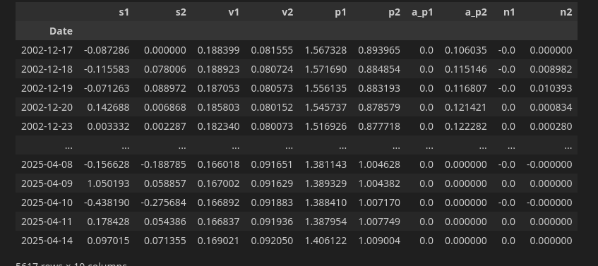
Creating a df such that:
Analyzing the Volatility Targeting Results
Once we have created the matrix with all the information needed for our calculations, we will visualize the P1 for SPY and P2 for TLT estimators on this occasion.
data[['p1','p2']].dropna().plot()
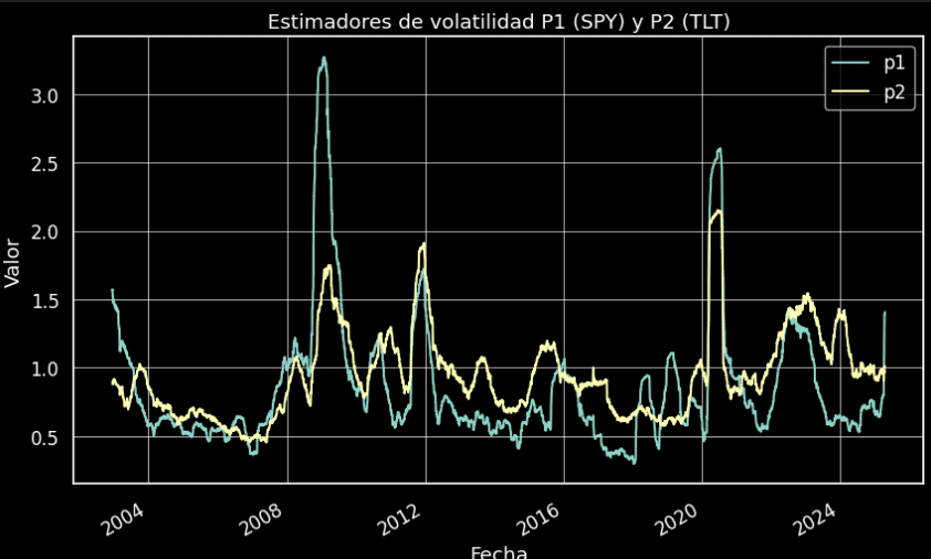
The volatility of the SPY asset is significantly higher than that of the TLT asset. However, an anomaly appears in the data due to interest rate changes in an inflationary economy, where the realized volatility of US Treasury fixed income is observed to be even higher than that of SPY. This is a very particular situation.
Now let's analyze what our model's weights would look like over time.
data[['a_p1','a_p2']].plot()
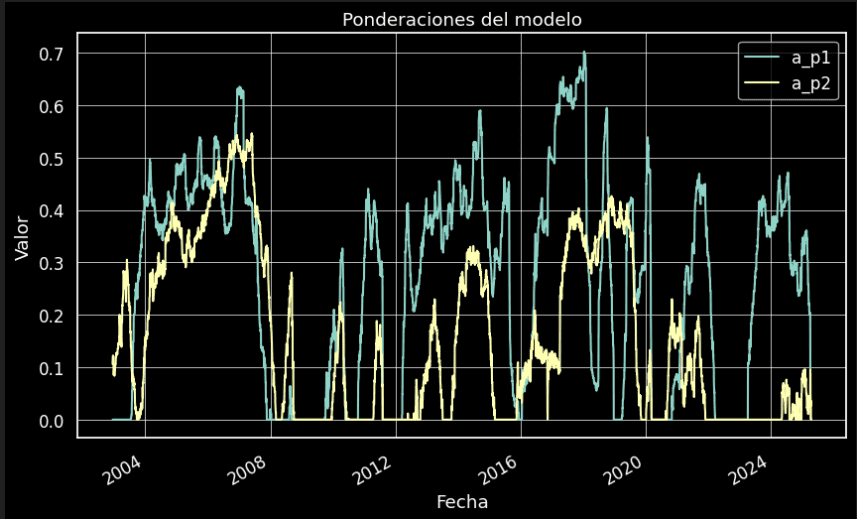
This method seeks to reduce portfolio volatility, focusing only on calm market periods. The model's predictive power is low, so it is not recommended for making long-term investment decisions. Nevertheless, the model's main advantage lies in its ability to adapt to the environment, as it seeks exposure and even leverage when it deems appropriate, and can hold very low weights, or even exit the market entirely, during high-volatility periods.
Let's add the two weights together to analyze whether there are moments when the model is out of the market or using leverage.
(data['a_p1'] + data['a_p2']).plot()
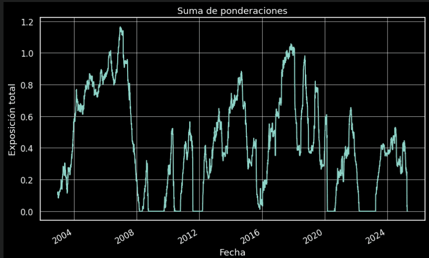
As you can see in the chart, the model generally stays below its maximum level without using leverage, although at certain specific moments it adopts a leveraged strategy. All the conditions for productive leverage can be defined within the model itself, but given the introductory nature of this article, the model will not be constrained in this regard.
Combining Returns with Asset Allocations
Now that we have confirmed that the fundamental premises underlying this model hold—that is, its ability to adapt to market volatility through volatility targeting mechanisms—we can move on to the next step.
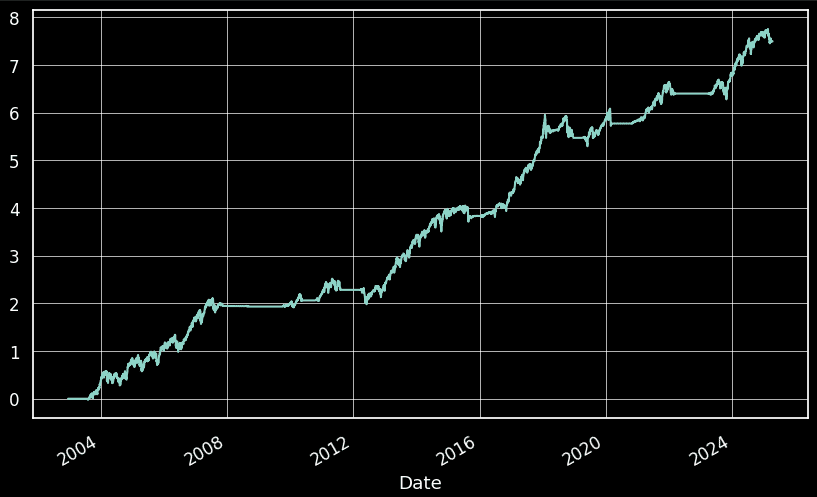
We will calculate the equity curves for each asset separately. We'll start with ST1 (SPY).
data['n1'] = data['a_p1'] * data['s1']
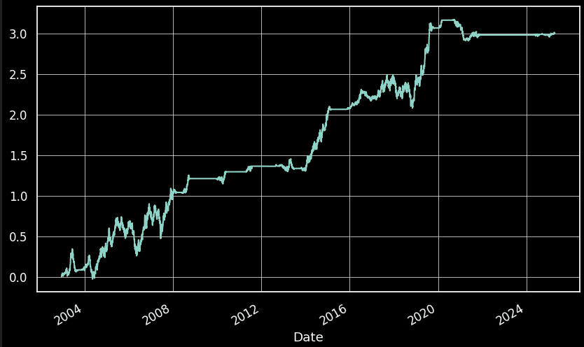
After applying Volatility Targeting, the procedure for calculating the equity curves is extremely simple: the percentage returns are multiplied by the corresponding weight. Below, we present the results obtained for the SPY asset:
And for the TLT asset:
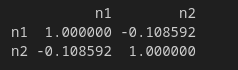
To better determine whether these two assets behave similarly or differently, we will run a correlation test. We expect to find values that do not exceed 0.2 or fall below -0.2. Furthermore, with Volatility Targeting the volatility of both assets has been adjusted.
data[['n1','n2']].corr(method='kendall')
Final Result – Volatility Targeting
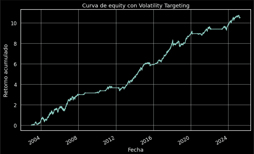
To visualize the results of the two portfolios, we simply need to add them together. The resulting curve after applying Volatility Targeting would be as follows:
(data['n1'] + data['n2']).cumsum().plot()
One of the most reputed managers, who built his empire on the concept of volatility targeting, is Ray Dalio. His fund applied a concept derived from volatility targeting. He used a technique known as Risk Parity.
Resources:
https://www.ecb.europa.eu/pub/financial-stability/fsr/focus/2020/html/ecb.fsrbox202005_02~f6616db9be.en.html
If you're looking to understand realized volatility, we recommend you check out this article.
If you're looking to understand implied volatility, we recommend you check out this article.
If you want to understand the three most common uses of volatility, we recommend you check out this article.
Extension for Members
In the following section, exclusively for members of our army, we will advance in volatility targeting at the asset level and at the strategy level. We will delve into the methods for adjusting our target, which can be reused as a foundation to get started with volatility targeting methods.
Volatility Targeting – At the Asset Level
Within portfolio management, there are three relevant levels of risk management, schematically:
- At the Portfolio Level: Where the goal is to control the volatility of a multi-strategy portfolio and enable tactical switching.
- At the Strategy Level: Where the goal is to target the volatility within a single strategy.
- At the Asset Level: Where the goal is to adjust the weighting of the asset within the strategy, across the various assets of the portfolio.
Although there are many situations where it is not possible to distinguish between different risk levels due to the hierarchical structure of risk baskets.
For example, multiple strategies (such as different moving average crossovers) can be considered as mean reversion or as momentum. This can depend on the trader's subjective preferences, or on exposures to the covariance structure, both in empirical and theoretical forms.
We will program a block that is usable at both the strategy level and the asset level, where we target conditional volatilities as the sole exposure factor.
When we refer to exposure, we do not have a narrowly defined concept of it. We consider exposure not only to returns, but to any other estimable factor of the strategy or asset we are analyzing, or even a combination of them.
These would be some of the objectives for which you should control exposure within the portfolio:
- Alpha (From the EV standpoint)
- Nominal value of the exposure
- Risk exposure as such